
We all know that HF Ionospheric propagation is the main variable that permits (or denies) radio communication. The principal HF system factors - propagation, antenna gain and transmit power - are the major factors in system effectiveness, and fig. 1 shows the relative effect of these variables.
There's not much we can do about propagation loss, except to use a software program to predict its effect. And we know that we can increase transmit power, within limits, to talk farther. But antenna gain is a factor we can control, and look at the possibilities - as much as 20 dB is available to us! And with a cooperative buddy at the receive end of the circuit, that's as much as 40 dB! Just think what that means: If we change to an antenna with 20-dB more gain, our 100-watt transmitter would operate with the equivalent power of 10,000 watts! Is it any wonder that hams spend a good part of their time selecting and optimizing their antennas? Clearly, having the right antenna is key to good station performance.
HOW DO ANTENNAS WORK?
Selecting your antenna is perhaps the most difficult task in constructing a ham station. And yet, antenna type, site and gain variations can influence station performance more than any other parameter. When we first studied for our ham licenses, we learned about isotropic antennas - those imaginary point sources floating out there in free space. Isotropic antennas are wonderful, as they emit equal amounts of radiation in all directions and we can specify their gains. Wow! Just what we need! Unfortunately, they don't exist, and we are constrained by real-world constructs that we erect somewhere near our ham shack.
But there are myriads of antennas to choose from, and we can examine the ways in which practical antennas really work. Let's begin by conducting a gedanken experiment-a thought experiment. Imagine that we take an isotropic antenna and bring it down to earth. We see a large sphere resting on the ground with an energy source, our transmitter, at its center point with radiation going out in all directions.
But real antennas don't work that way. They sit on the ground (or on a tower close to the ground) and radiate in directions above ground. (In theory, certain antennas like short verticals form an image antenna below ground, but let's skip that refinement for now.) So in our experiment, let's change to a hemisphere resting on the ground with a transmit source at the center, also on the ground. Now imagine our hemisphere is a rubber balloon with gas inside. A giant comes along and pokes his big finger into the side. What happens? The balloon depresses under his finger, and expands everywhere else. The transmit power remains constant, but the radiated power decreases under the giant's finger and increases in other directions.
Let's continue our experiment. Imagine a giant with lots of fingers and maybe many hands. If he is smart, he can poke and squeeze the balloon in ways that will concentrate the radiation in only one direction. Presto! We have a directional antenna! But we see that to get more gain in one direction - the main beam - we must sacrifice gain in other directions. Sometimes that is an intentional advantage, as in the case of a log periodic antenna that emits most of its energy in the main beam while it suppresses unwanted signals in the backward direction.
What have we learned so far? Well, our unmolested balloon antenna has equal gain in all directions, and it will expand - have greater gain - only if we increase transmitter power. If we want more gain in a given direction, we must poke and squeeze the hemisphere. That is, we must construct a more complex antenna that will concentrate power in one direction at the expense of radiation elsewhere. And it's tough to make a truly omni-directional antenna. There will always be some compromise.
And we haven't yet talked about broadband operation. Most antennas work best over a limited frequency range. If we design a simple antenna, like a horizontal dipole, it is usually cut for the lowest band we wish to use. At higher frequencies it will work, but our giant starts poking his fingers again and the radiation patterns are anything but uniform and omni-directional.
ANALYZING ANTENNAS
To make sense out of this mess, we would really like to have a tool that helps us visualize the antenna's performance. Fortunately, such tools exist and usually focus on two parameters: radiation pattern and gain. Since patterns are seldom omni-directional in all planes, we speak of directivity - the direction in which the antenna's radiation is concentrated. And directivity gain usually refers to maximum relative gain, Gmax - the gain in the direction of maximum radiation valued with respect to that of an isotropic radiator, stated in dBi.
Over the years, standards have been developed for visualizing antenna patterns and gains. ACE-HF PRO includes an antenna analysis program called HFANT that graphs the antenna's radiation pattern in two views. For example, fig. 2 (below) shows the azimuthal (horizontal) and elevation (vertical) patterns for a typical half-wave horizontal dipole antenna mounted one-quarter wave above ground. The antenna is 40 meters long, making it resonant in the 80-meter band, and is mounted about 20 meters above average ground. The antenna has a maximum gain (Gmax) of 5.7 dBi. (The charts show relative gain patterns drawn with respect to Gmax.)
Fig. 2a - 80-m Horizontal Dipole Antenna at 3.75 MHz:
(click to view full-size version)
Fig. 2b - 80-m Horizontal Dipole Antenna at 3.75 MHz:
(click to view full-size version)
In the dipole example, the azimuthal pattern when viewed from overhead is nearly omni-directional. That is, the radiated energy is nearly the same in all directions. This makes it a good general-purpose antenna for 80-meter operation. Physically, the antenna wire runs between the 90 degree and 270 degree angles of the azimuthal chart and the maximum emission is broadside to the antenna. In the end-fire directions, emission is seen to be down about 7.5 dB with respect to the maximum gains at 0 degrees and 180 degrees. The convention is to always draw such charts with their maximum azimuthal gain at 0 degrees - at the top of the graph. Of course, you may erect your dipole antenna at any physical angle, which is usually constrained by available property limits or by the presence of convenient trees!
In the ACE-HF PRO software, the azimuthal angle of maximum emission - at 0 degrees in fig. 2 - is assumed to point at a 0 degree bearing, i.e. at true North. Thus, one can think of the azimuthal graph as being laid out at the four compass angles, where 90 degrees is East, and so on. But in the software, the user can specify the antenna azimuth at both ends of a circuit. For example, if you have a directional antenna like a Yagi antenna, you can rotate the antenna's azimuth in the software just as you would when operating your station. In effect, that points the 0 degree angle of the azimuthal chart to a specified bearing angle. And to make things easier, there is a 'point at button' you can check that automatically points the antenna at the distant station. If you have a fixed antenna, then the software's azimuth angle should be set in the physical direction of maximum emission. For the dipole, that would be the broadside angle.
Let's continue with our antenna analysis. Fig. 3 (below) shows patterns for the same dipole antenna, except that we changed the driving frequency to 14.2 MHz. The antenna still works, but the patterns are rather different, and the maximum gain at this frequency has fallen to -1.2 dBi.
Fig. 3a - 80-m Horizontal Dipole Antenna at 14.2 MHz:
(click to view full-size version)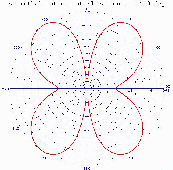
Fig. 3b - 80-m Horizontal Dipole Antenna at 14.2 MHz:
(click to view full-size version)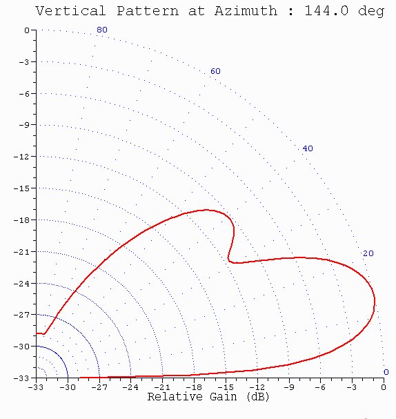
The first things to notice are the deep nulls in the four azimuthal directions. (The Gmax angle is oriented to the top of the chart at its design frequency, which in this case was 3.75 MHz.) The nulls are an important finding, because they can explain why we might have problems with circuit paths oriented along the null directions. This multi-lobing, as it's called, is caused by the multiple wavelengths that can exist on a dipole antenna that is resonant at a lower frequency. All antennas exhibit variable patterns as frequency changes, which explains why it is so difficult to design a truly wideband antenna.
Now let's look at the right-hand charts of the figures. In fig. 2, the vertical (elevation) pattern shows a slice of the pattern from horizontal (0 degrees on the circular elevation axis) to 90 degrees at the zenith. This chart shows why horizontal dipoles are good choices for NVIS (Near Vertical-Incidence Skywave) circuits where the circuits are very short and the ionospheric reflection angles are close to the zenith. In fig. 3, however, the maximum radiation occurs at a low, 14 degree, angle, so this dipole operated in the 20-meter band would be a poor NVIS antenna.
Analyzing another simple antenna, the vertical monopole, fig. 4 (below) shows the patterns for a quarter-wave, base-insulated vertical where height depends on the lowest frequency of operation. The lowest practical frequency for such designs usually depends on one's property size, because tall masts must be guyed. In this case we specified a 20-meter height (about 66 feet), which is about right for operation on 80 meters.
Fig. 4a - 80-m Vertical Antenna at 3.75 MHz:
(click to view full-size version)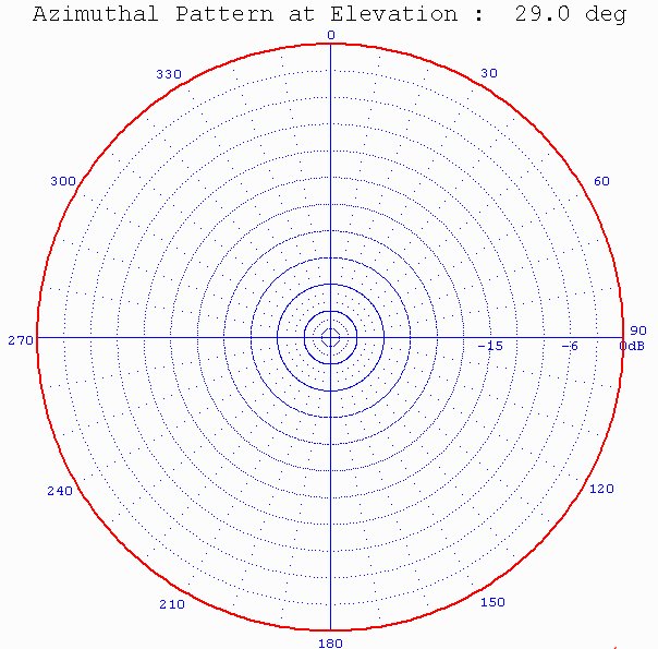
Fig. 4b - 80-m Vertical Antenna at 3.75 MHz:
(click to view full-size version)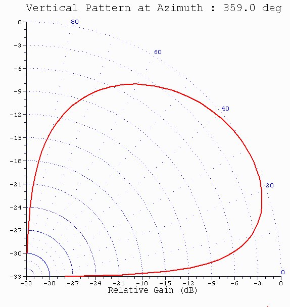
As expected, this is an omni-directional antenna. That is, radiation is uniform in all horizontal directions. In this example, Gmax is -2.5 dBi at 3.75 MHz when the antenna is installed over poor ground. When erected over wet ground, Gmax increases to +0.9 dBi, but the antenna is still not very efficient. It is for this reason that vertical monopoles are usually equipped with a copper ground plane - a series of copper wires radiating from the base and extending, ideally, to a length equal to the antenna's height. When higher powers are involved, as with AM broadcast antennas, a copper-mesh screen is usually added at the base to further reduce ground losses, and the radial ground wires are brazed to the edge of the ground screen. The need for a good, high-conductivity, ground system is common to all vertically polarized antennas. But in this example, the copper ground system is omitted and only the earth's conductivity and permittivity values were specified.
Note that the vertical pattern shows essentially zero emission at the zenith, indicating that this design would be poorly suited for NVIS communications. The position of Gmax at 29 degrees in elevation shows that the vertical would best be used in medium- to long-distance circuits.
Fig. 5 (below) repeats the patterns for a 20-meter high vertical monopole, except that in this case the antenna is driven at 14.2 MHz. The azimuthal pattern is still omni-directional - it could hardly be anything else with a single vertical element. The elevation pattern has changed slightly, but is still essentially the same. The electrical length has increased from 1/4-wavelength to nearly a full wavelength at 14.2 MHz, and as a result Gmax has risen to 1.9 dBi over poor earth and 4.5 dBi over wet earth. However, driving-point impedance and VSWR may oscillate over an excessive range as frequency increases, which is why some proprietary verticals add traps and other lumped-constant components to smooth their wideband performance.
Fig. 5a - 80-m Vertical Antenna at 14.2 MHz:
(click to view full-size version)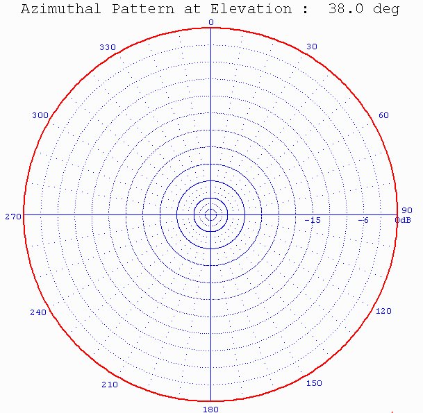
Fig. 5b - 80-m Vertical Antenna at 14.2 MHz:
(click to view full-size version)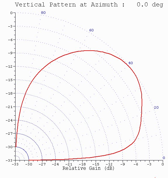
Verticals that are less than a quarter-wavelength in height at the lowest frequency are termed electrically short antennas. Short verticals erected in limited spaces, and the whips we mount on our cars, are usually less efficient. (Remember the old guide: "Antennas that stick out work better!") Their driving-point impedances are also capacitive, so to tune the antennas, series inductors called loading coils are often added at the base. Such coils increase the antenna's effective length, lower the feed-point impedance and thus reduce the high voltages than can exist with such whips. (Nevertheless, touching an energized whip can result in a nasty shock!) Modeling such antennas is more difficult because the model should include the orientation of the antenna (some mobile operators tie the tips down avoid breaking them off in tunnels), lumped-constant components such as loading coils, and the presence of the vehicle's metallic body.
It is important to know that the figures just illustrated show only the best-case radiation patterns. Let's go back to our gedanken experiment and look again at our hemisphere of radiation. Imagine that there are 360 planes of radiation emerging at horizontal intervals from the energy center. Assume that these radiate out at one-degree intervals and each plane covers angles from zero to 90 degrees in elevation. Along each of these 360 slices we can designate 91 incremental points in elevation. We can think of each of the points as the end of an energy vector, and the ends of all those vectors form the extent of radiated energy in three-dimensional space. Thus, there are 360 x 91 = 32,760 points of gain along a 3D surface if we limit ourselves to one-degree intervals in both dimensions. The surface is an undulating, irregular connection of gain values, the maximum of which is called Gmax.
The patterns produced by HFANT show only a single pattern amongst those that actually exist. The software first finds the Gmax value out of 32,760 possibilities. It flags that point and reports that Gmax exists at a certain azimuthal and elevation angle. Fig. 2 shows that the azimuthal pattern is drawn at a 49 degree elevation angle, and the vertical pattern is drawn for an azimuth of 360 degrees. This convention of drawing relative gain patterns with respect to Gmax is a powerful method for comparing antennas and has become an industry standard. But there are many, many other patterns that could be drawn if we have the right tools. (See 3D Antenna Charts near the end of this article.)
Fig. 6 (below) shows the radiation pattern charts for a 10-m OptiBeam 3-stack Yagi Array with a gain of 19.6 dBi at 4 degree elevation. The Yagis of the stack are set at 150, 100 and 50 feet above ground and rotate together to specified azimuths.
Fig. 6a - 10-m OptiBeam Yagi Stick Antenna at 28.4 MHz:
(click to view full-size version)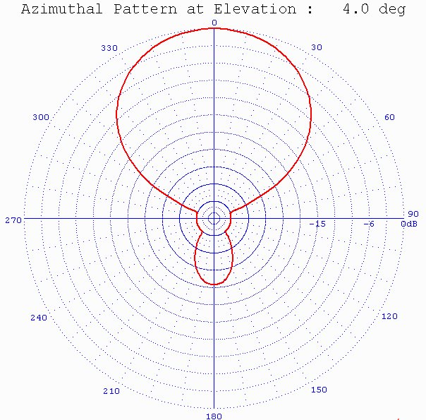
Fig. 6b - 10-m OptiBeam Yagi Stick Antenna at 28.4 MHz:
(click to view full-size version)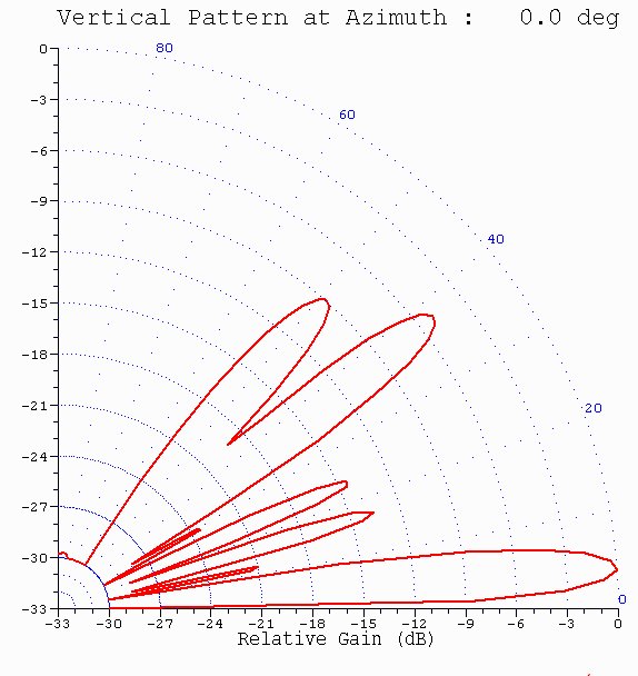
This antenna has a very high directional gain and the main beam is set at a low elevation angle. It also has an exceptional beamwidth (the angular azimuthal width of the pattern at the -3-dB points) of nearly 60 degrees. This antenna is ideally suited for worldwide DX operation.
ANTENNAS IN SYSTEM SIMULATIONS
As you can see, one can build an entire hobby out of looking at different antenna models. It's fun and instructive, and there are a lot of models to look at. Why do we do it? First, we want to see how effective our existing antenna might be. Or, we may be considering another antenna, and modeling it in software is a try-before-buy method that doesn't cost much. And if we have ACE-HF PRO, we are interested in simulating our HF system to find best frequencies, to determine our coverage areas, and to optimize our operation in general. Having the correct antenna model is key to all of those needs.
ACE-HF PRO (version 2.05) comes with more than 800 different antenna models, and many of these may be modified using the HFANT program. Fig. 7 (below) shows how those models are used in the software.
Fig. 7 - Antenna Modeling Methods in ACE-HF PRO:
(click to view full-size version)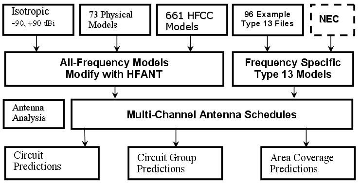
If nothing else is known about a contact's antenna, use an Isotropic antenna with an assumed gain. If the antennas are of common types, you can use physical, i.e. mathematical, models that may be modified using HFANT. More accurate models may be made using NEC software such as NEC Win PLUS+, and saved as ACE-HF Type 13 gain-table files.
(Note: Numerical Electromagnetic Code (NEC) software was created by Laurence Livermore Laboratories to model very complex antenna structures and their surroundings by dimensionally specifying each antenna wire and structure using method-of-moments computations. Each wire within the antenna design is specified by the physical (XYZ) location of each end, and a line is drawn between the two ends to represent an antenna element. The process is repeated until all antenna elements and surrounding surfaces are described and computations then proceed. The resulting NEC model may then be analyzed vs. frequency. Common output parameters include both vertical and elevation patterns, gain values at each vertical and elevation angle, antenna input impedances and VSWRs.)
Type 13 files are frequency-specific, and for best accuracy a separate file should be generated for each frequency. ACE-HF automatically runs ten frequencies for each prediction. When separate Type 13 files are used, they may be individually specified for different bands with user-made multi-channel antenna schedule files.
Don't worry about all those complex pattern lobes and nulls when you make a system simulation. ACE-HF will account for them automatically, and will compute the right signal strength at the receiver.
OPTIMIZING ANTENNA LAUNCH ANGLES
A special ACE-HF chart may be used to be sure your antenna is appropriate for a particular circuit. For maximum effectiveness, the launch (take-off) angle of your antenna's main beam should coincide with the elevation angle of the Most Reliable Mode (MRM) of the propagation path. An example chart is shown in fig. 8 (below), where I analyzed a circuit from my station near Seattle to Denver, Colorado.
Fig. 8 - 40-m Yagi Launch vs. MRM Elevation Angles:
(click to view full-size version)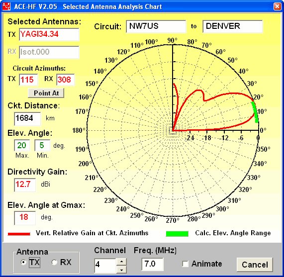
There is a wealth of information in such analysis charts. The circuit path is shown at the top, along with the antennas that were selected at both ends of the circuit. The antenna azimuth settings are given next, along with the circuit distance. The range of the MRM elevation angles throughout a 24-hour day are also given, together with the directivity gain (Gmax) and the elevation angle at Gmax.
This figure compares the elevation angle range (in green) of the MRM vs. the antenna's main beam launch angle (in red) at 7.0 MHz. It is surprising how much insight one gains when the chart is animated through the 2-30 MHz frequency range.
TYPE 13 ANTENNA MODEL ANALYSIS FOR ACCURATE SYSTEM SIMULATION
Although mathematical antenna models are easy to modify and use, the most accurate system simulations result when NEC Type 13 models are used. Mathematical models are somewhat generic, and it would be nearly impossible to generate such models for every conceivable case. NEC models, on the other hand, can be tailored by the user for one's particular situation. As a simple example, perhaps a Amateur Radio operator erects a simple long-wire antenna having a dogleg and sloping down from a treetop to his house. Such an unusual arrangement would be unlikely to be found in the model list; a custom antenna model is needed and a Type 13 file could be produced.
ACE-HF contains a special set of charts to illustrate patterns from Type 13 antenna models. Patterns for a really good directional antenna, the Sample13.13 model included with the software, are shown in fig. 9 (below). This model is for a large fixed antenna used in HF broadcasting service, and is a aperiodic dipole array with a reflecting curtain, mounted vertically and suspended between towers. The array consists of four rows of elements in four stacks mounted 0.5 wavelength high. Phased feeds to various elements can slew the main beam to different azimuths although the antenna is fixed.
Fig. 9 - HF curtain array antenna for 11.85 MHz:
(click to view full-size version)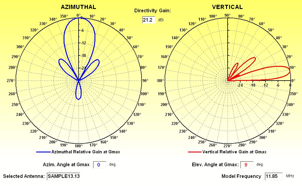
This example is shown to suggest what beautiful and well-controlled patterns one can achieve when the antenna design is complex. (Compare it with the Yagi Array in fig. 6.) It is unlikely that an amateur operator would erect such a huge array, but wouldn't it be fun?
(Note: I have a friend who worked years ago for Continental Electronics, the maker of large HF broadcast transmitters. They had a curtain array for testing purposes, and some of the ham employees made worldwide contacts driving the curtain with a keyed grid-dip meter!)
The ACE-HF chart shows a directivity gain of 21.2 dBi at an elevation angle of 9 degrees for this antenna. A set of 1-MHz interval gain-table files are included with the ACE-HF PRO V2.05 installation CD. The selected antenna was a terminated folded-dipole antenna 50-foot long elevated 15 meters above ground. Fig. 10 (below) shows a sampling of these Type 13 analysis charts in 4-MHz steps. (In the software, the series can be animated in 1-MHz steps from 2 through 30 MHz.)
Fig. 10 - Terminated folded dipole antenna at 2 to 30 MHz (animated):
(click to view full-size ANIMATED version)
While these charts are fascinating, each pair still represents a single slice through our imaginary antenna balloon. Wouldn't it be nice if we could create a three-dimensional figure, as we did in our gedanken experiment?
3D ANTENNA CHARTS
For centuries, cartographers have sought to illustrate a three-dimensional, spherical globe on two-dimensional paper. (See "The Round Earth on Flat Paper", National Geographic Society, 1947.) People have struggled with various projections, but it seemed there was always some distortion, some stretching of the land, that made the maps look strange.
The ACE-HF folks struggled with the same problem in considering antenna charts, and it would be great if we could have a 3D spherical antenna chart that would visualize our gedanken experiment. On the flat computer screen, as on the paper of this article, a compromise was reached. Figs. 11 and 12 (below) show three-dimensional charts for two of the antennas discussed, from the ACE-HF PRO V2.05 software.
Fig. 11 - 3D chart of TF dipole antenna at 10 MHz:
(click to view full-size version)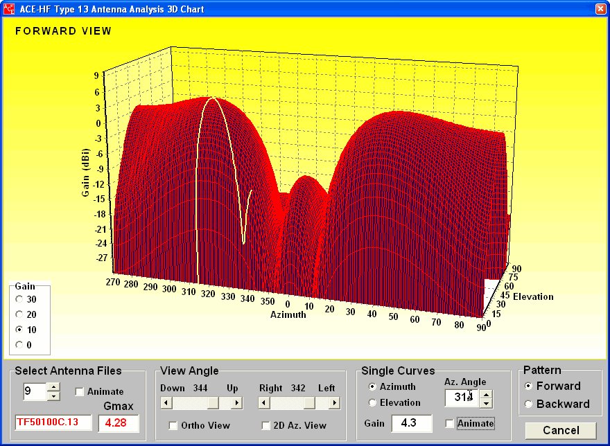
Fig. 12 - 3D chart of OptiBeam yagi stack at 28.4 MHz:
(click to view full-size version)
The 3D charts are lots of fun to play with. You can change the viewing angle, show different projections and even shift between forward and backward antenna patterns. And you can animate a single slice through the figure as a function of azimuth or elevation angle. In fig. 11, the yellow line shows the slice at 314 degrees azimuth where Gmax of 4.3 dBi occurs at the top of the diagram. In fig. 12, the yellow line shows the Gmax slice at an elevation of 4 degrees.
THE BOTTOM LINE
I can guarantee that once you play with all these charts, you will be a lot smarter about antennas. But the bottom line is to show the effectiveness of our radio station. To answer that question, I ran ACE-HF area coverage maps for my station in Brinnon, WA to see how different antennas would affect my communications range. Fig. 13 (below) shows 40-meter coverage at 02 UTC from a quarter-wave vertical monopole, while fig. 14 (below) shows coverage from a two-stack array of 4-element Yagis mounted at 75 and 125 feet above ground, pointed at a 90 degree azimuth angle. The conclusions are obvious, and just wait until you animate these maps through 24 hours with the ACE MOVIE program!
Fig. 13 - NW7US 40-m coverage with quarter-wave vertical:
(click to view full-size version)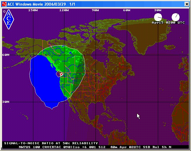
Fig. 14 - NW7US 40-m coverage with 2-stack yagi array:
(click to view full-size version)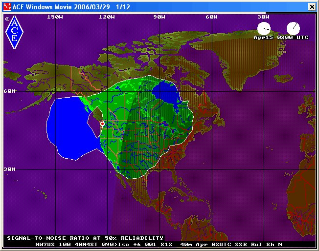
Have I learned anything from my analysis? Yes! Do I want a new antenna? You bet!
Now, you also know how to explore the right antenna for your application, before you buy the antenna or spend time constructing the antenna. Once you discover the right antenna by using the modeling features of ACE-HF, you can spend the time to construct the antenna, and then be armed for success.
Monday, June 20, 2011
Antennas are the key!
How do we make our HF ham stations work more effectively? If you are new to ham radio - or a technician-class ham planning to venture into HF under the new rules - you want to talk to as many other stations as you can. If you are seasoned operator, you want a higher score in that contest. Either way, you really don't want to waste time calling, "CQ." That's fun the first time or so, but isn't it better to know in advance how you can quickly make your contacts? To develop that confidence, one must understand the radio system in its entirety.
Subscribe to:
Post Comments (Atom)
No comments:
Post a Comment